Intro to NumPy & Linear Algebra — Follow-Along

Try me

This notebook blends NumPy basics with Linear Algebra in NumPy. Use the predict → run habit: mentally predict outputs, then execute to check.

0) Setup

Import NumPy and create a random generator for reproducibility.

import numpy as np

Introduction

Motivation

• AI and machine learning combine statistics and mostly linear algebra

• Key enabler efficient and scalable linear algebra operations with large data

• Bridge the gap between mathematical language and programming languages

Objectives

• Understand the mathematical engine that drives so much of modern tech: Array programming

• Bypass (slow and computationally inefficient) basic for loops.

• Do so through the lens of linear algebra

• Find links between mathematical modeling and programming

Intro for Non-Programmers (I)

• Numpy: Python holy grail for array programming

• Array programming let us bypass for loops and implement faster operations with Matrices and vectors

• Basic terminology:

  • A simple list of numbers, mathematically is just a vector. In numpy, we call it a 1D array, it has exactly an axis, or dimension.

  • If you have something like a spreadsheet, a table, mathematically, we call it a matrix. In Numpy, we call it a 2D array, it has two axis or dimensions

  • Dimensions are called axis: We can have an arbitrary number of dimensions or axis in a Numpy array

  • The rank tells us the number of dimensions. The shape, the number of elements

Intro for Non-Programmers (II)

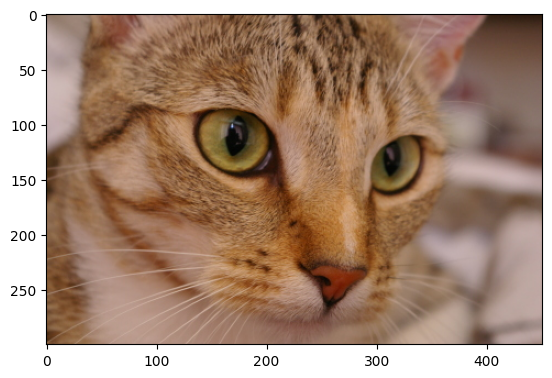
• Think of a color image, with width, height, and 3 color channels.

• We can fit the data into an array of rank 3: Height, width, and color

• The shape is 300x451x3 (300x451 image times 3 colors)

from skimage import data
from matplotlib import pyplot as plt
cat = data.chelsea()
plt.imshow(cat)
print(cat.shape)

(300, 451, 3)

Intro for Non-Programmers (II)

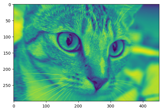
• We can get a color channel for instance just by slicing the image.

plt.imshow(cat[:,:,1]) # Only Green

<matplotlib.image.AxesImage at 0x1150ff750>

Agenda

• Intro 25 minutes

• Numpy basics 30 minutes

• Linear algebra 30 minutes

Part A — NumPy Basics

Core concepts: creation, shapes/dtypes, indexing & slicing, boolean masks, broadcasting, vectorized ops, aggregations.

Key ideas

• Numpy arrays: multidimensional, fixed-type containers for numbers.

• Array programming: think in terms of whole arrays, not elementwise loops.

A1) Creating arrays

• From Python objects: np.array([1,2,3])

• Ranges/grids: np.arange, np.linspace

• Filled arrays: np.zeros, np.ones, np.full, np.eye

• Random: random.int, random.normal

• dtype used to force or read the type

a = np.array([1, 2, 3])
b = np.arange(0, 10, 2)        # step range
c = np.linspace(0, 1, 5)       # 5 points in [0,1]
Z = np.zeros((2,3))
O = np.ones((3,2))
F = np.full((2,2), 7.5)
I = np.eye(3)
R = np.random.normal(loc=0, scale=1, size=(3,2))  # Random values with normal distribution

print("a:", a, a.dtype)
print("b:", b)
print("c:", c)
print("Z:\n", Z)
print("I:\n", I)
print("R:\n", R)

a: [1 2 3] int64
b: [0 2 4 6 8]
c: [0.   0.25 0.5  0.75 1.  ]
Z:
 [[0. 0. 0.]
 [0. 0. 0.]]
I:
 [[1. 0. 0.]
 [0. 1. 0.]
 [0. 0. 1.]]
R:
 [[ 0.21647229 -1.00414296]
 [ 0.14917009 -1.82099297]
 [-0.91626809  0.70258613]]

# Challenge. np.random.randint(low,high,shape) creates a numpy array of any shape with values from low to high. For instance, np.random.randint(0,5, (2,3)) creates a numpy array of shape 2x3 with values between 0 and 5.
# Use this info to create an array of size 128x128 with random bits

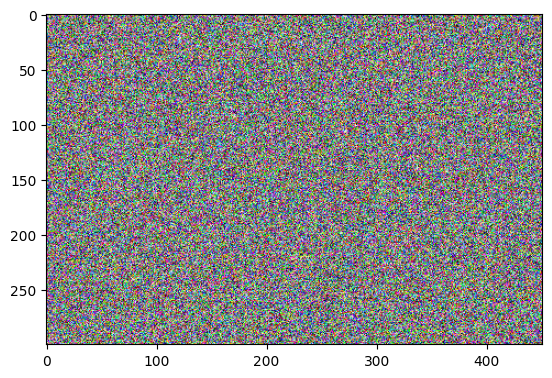
# Challenge. Look at the cat example in the introduction. Use the function random to create an image of the same size as cat, but with random integer values drawn from 0 and 255, and then plot it.

<matplotlib.image.AxesImage at 0x11403ee90>

A2) Shape, dtype, size

• .shape, .ndim, .size, .dtype, .itemsize

• astype converts dtype

M = np.random.normal(0, 100, size=(3,4))
print("shape:", M.shape, "| ndim:", M.ndim, "| size:", M.size)
print("dtype:", M.dtype, "| itemsize:", M.itemsize, "bytes")
print("astype float32:\n", M.astype(np.float32))

shape: (3, 4) | ndim: 2 | size: 12
dtype: float64 | itemsize: 8 bytes
astype float32:
 [[ -87.16807   136.74026   177.31474  -174.9163  ]
 [ -28.215887   97.507545   -7.764087   64.47249 ]
 [-131.9176   -162.41922   219.6428     85.892395]]

A3) Indexing, slicing, boolean masks

• 1D: x[i], x[i:j:k]

• 2D: A[i, j], A[i, j1:j2], row/col slices

• Masks: mask = (A % 2 == 0) → A[mask]

x = np.arange(10)
A = np.random.normal(0, 20, size=(4,5))
print("x:", x)
print("x[2:8:2]:", x[2:8:2])
print("A:\n", A)
print("A[1, :]:", A[1, :])
print("A[:, 2]:", A[:, 2])

mask = (A > 10)
print("mask as 0/1:\n", mask.astype(int))
print("A[mask]:", A[mask])

x: [0 1 2 3 4 5 6 7 8 9]
x[2:8:2]: [2 4 6]
A:
 [[ 40.29040845  11.2099828   12.6670429  -19.53236574  24.9790349 ]
 [ -1.32035248  -5.32789079  -0.6299237    4.87824025 -15.86258631]
 [-20.80897509  28.79256532   3.99200466   6.43368619  -7.87346429]
 [-12.4336586   -4.08926711  19.30743726  12.50232581   5.03352625]]
A[1, :]: [ -1.32035248  -5.32789079  -0.6299237    4.87824025 -15.86258631]
A[:, 2]: [12.6670429  -0.6299237   3.99200466 19.30743726]
mask as 0/1:
 [[1 1 1 0 1]
 [0 0 0 0 0]
 [0 1 0 0 0]
 [0 0 1 1 0]]
A[mask]: [40.29040845 11.2099828  12.6670429  24.9790349  28.79256532 19.30743726
 12.50232581]

# Mini challenge
# Print the two first rows of A

# Use a mask to find the values of A that are lower than 0

A4) Broadcasting

• Fancy word, just extends a constant or array so that it matches the shape of another array

• Align shapes from the right; dims are compatible if equal or either is 1.

B = np.ones((3,4))
row = np.array([1, 0, -1, 2])     # shape (4,)
col = np.array([[10],[20],[30]])  # shape (3,1)

print("B:\n", B)
print("B + row:\n", B + row)   # across rows
print("B + col:\n", B + col)   # down columns

B:
 [[1. 1. 1. 1.]
 [1. 1. 1. 1.]
 [1. 1. 1. 1.]]
B + row:
 [[2. 1. 0. 3.]
 [2. 1. 0. 3.]
 [2. 1. 0. 3.]]
B + col:
 [[11. 11. 11. 11.]
 [21. 21. 21. 21.]
 [31. 31. 31. 31.]]

# Mini challenge: Assume the array below contains the prices of products of a portfolio. Each row represents a country and each column a product
prices = np.random.normal(2, 5, size=(30,40))
# Use broadcasting to add a flat 1 euro export tariff to your prices.

A5) Vectorized ops, ufuncs, aggregations

• Elementwise: `+ - * / **`

• Ufuncs: np.sqrt, np.exp, np.clip, np.where

• Aggregations: np.sum, np.mean, np.std with axis=

• axis determines in which dimension or axis the operation will be performed.

• These are much more efficient than for loops!

X = np.linspace(-2, 2, 5)
print("X:", X)
print("X**2:", X**2)
print("sqrt(abs(X)):", np.sqrt(np.abs(X)))
print("where(X>=0, 1, -1):", np.where(X>=0, 1, -1))

G = np.random.randint(0,5, (2,3))
print("G:\n", G)
print("sum all:", np.sum(G))
print("mean per col:", np.mean(G, axis=0))
print("std per row:", np.std(G, axis=1))

X: [-2. -1.  0.  1.  2.]
X**2: [4. 1. 0. 1. 4.]
sqrt(abs(X)): [1.41421356 1.         0.         1.         1.41421356]
where(X>=0, 1, -1): [-1 -1  1  1  1]
G:
 [[4 2 4]
 [0 3 1]]
sum all: 14
mean per col: [2.  2.5 2.5]
std per row: [0.94280904 1.24721913]

# Mini challenge.
# do the sum in each axis (with axis = 0, axis = 1, and axis = 2) in the following numpy array to understand the axis
axis_test = np.ones((2,3,4))
print("axis_test:\n", axis_test)
print("sum in axis 0:\n", axis_test.sum(axis=0))
## TODO: Complete and do the sum in the other two axis. Analyse the results

A-PI Cards (predict; then run the check cell)

Card A1 — Slicing vs copying

A = np.arange(9).reshape(3,3)
B = A[0, :]      # view or copy?
B[0] = 99

What changes in A?

A = np.arange(9).reshape(3,3)
B = A[0, :]
B[0] = 99
print("A:\n", A)

Card A2 — Mask + broadcasting

X = np.array([[-1,0,1],[2,-2,3]])
X[X<0] = X[X<0] + 10

Predict final X.

X = np.array([[-1,0,1],[2,-2,3]])
X[X<0] = X[X<0] + 10
print(X)

Card A3 — Axis confusion For A.shape == (4,5,6), what shape is np.sum(A, axis=1)?

A = np.zeros((4,5,6))
print("sum axis=1 ->", np.sum(A, axis=1).shape)

Part B — Linear Algebra with NumPy

B1) Dot (scalar) product

Key Concepts

• A vector is an ordered array of numbers (1-D array). 1-D means it has only one axis or dimension.

• For instance, the vector \(v=[4,5,6]\) has three elements, and the vector $w = [2, 3, 4, 5] has four elements.

• The dot product of two vectors is the sum of the products of their corresponding elements.

Mathematical notation:

For vectors \(c, v \in \mathbb{R}^n\) (the set of real-valued vectors of dimension \(n\)): \(\displaystyle c\cdot v = \sum_{i=1}^{n} c_i v_i\)

for instance, for \(c=[1,2,3]\) and \(v=[4,5,6]\) (\(n=3\), \(c,v \in \mathbb{R}^3\)):

\(c\cdot v = \sum_{i=1}^3{c_i*v_i} = 1*4 + 2*5 + 3*6 = 32\)

Implementation

⚠️ Summations are just like for loops in programming!

In Python, from scratch:

dot_product = 0
c = [1,2,3]
v = [4,5,6]
for i in range(len(c)):
    dot_product += c[i] * v[i]

In Python, using comprehensions:

dot_product = sum(c[i]*v[i] for i in range(len(c)))

In NumPy:

• a @ b (preferred)

• np.dot(a, b) (equivalent)

a = np.array([1.,2.,3.])
b = np.array([4.,5.,6.])
print("a@b:", a @ b)
print("np.dot:", np.dot(a,b))

B2) Matrix product (2-D @ 2-D)

Key concepts

• A matrix is a 2-D array (two axes/dimensions).

• Matrix dimensions: A is (m, p) if it has m rows and p columns.

• For instance:

\(A = \begin{bmatrix} 1 & 2 & 3\\ 4 & 5 & 6 \end{bmatrix}\)

has shape (2, 3) (2 rows, 3 columns).

A = np.array([[1,2,3],
              [4,5,6]], dtype=float)   # (2,3)
B = np.array([[1, 0],
              [0, 1],
              [1,-1]], dtype=float)    # (3,2)
C = A @ B
print("C shape:", C.shape, "\nC=\n", C)

• Matrix multiplication combines rows of the first matrix with columns of the second via dot products.

Example: \(A = \begin{bmatrix} 1 & 2 & 3\\ 4 & 5 & 6 \end{bmatrix}\) \(B = \begin{bmatrix} 1 & 0\\ 0 & 1\\ 1 & -1 \end{bmatrix}\)

Then:

\(C = A @ B = \begin{bmatrix} (1*1 + 2*0 + 3*1) & (1*0 + 2*1 + 3*-1)\\ (4*1 + 5*0 + 6*1) & (4*0 + 5*1 + 6*-1) \end{bmatrix} = \begin{bmatrix} 4 & -1\\ 10 & -1 \end{bmatrix}\)

Mathematical notation:

• If \(A\) is an \((m,p)\) matrix, then \(A \in \mathbb{R}^{m \times p}\).

• If \(A\) is an \((m,p)\) matrix, element at row \(i\) and column \(j\) is \(a_{ij}\).

• The matrix product \(C = A B\) of \(A \in \mathbb{R}^{m \times p}\) and \(B \in \mathbb{R}^{p \times n}\) results in \(C \in \mathbb{R}^{m \times n}\), where each element is:

\(c_{ij} = \sum_{k=1}^{p}{a_{ik}*b_{kj}} \quad \forall i \quad \forall j\)

(that is, the dot product of the \(i^{th}\) row of \(A\) and the \(j^{th}\) column of \(B\)).

Implementation

In Python, from scratch:

A = [[1,2,3],[4,5,6]]
B = [[1,0],[0,1],[1,-1]]
m = len(A) # A has two elements (rows), each one a list of 3 elements (columns)
p = len(B) # or p = len(A[0])
n = len(B[0])
C = [[0 for i in range(n)] for j in range(m)]
for i in range(m): # For each row of A
    for j in range(n): # For each column of B
        for k in range(p):  #  Do the dot product
            C[i][j] += A[i][k] * B[k][j]
print(C)

Using comprehensions:

C = [[sum(A[i][k] * B[k][j] for k in range(p)) for j in range(n)] for i in range(m)]

Using NumPy:

C = A @ B

# Playground: explore matrix product
A = np.array([[1, 2, 3],
              [4, 5, 6]], dtype=float)   # (2,3)
B = np.array([[1,  0],
              [0,  1],
              [1, -1]], dtype=float)      # (3,2)
C = A @ B
print(f"C shape: {C.shape}, C= {C}")

B3) Transpose & reshape

• 2-D transpose: A.T

• General axis permute: np.transpose(A, axes=...)

• Reshape without changing data: A.reshape(new_shape)

M = np.arange(1,13).reshape(3,4)
print("M:\n", M)
print("M.T:\n", M.T)

T = np.transpose(M.reshape(2,2,3), axes=(0,2,1))
print("permute axes shape:", T.shape)

v = np.arange(12)
print("v reshape (3,4):\n", v.reshape(3,4))

B4) Norms & vector length

np.linalg.norm(x) is L2 by default; ord=1 (L1), ord=np.inf (max). For rows/cols: use axis and keepdims=True.

x = np.array([3.0, 4.0])
print("L2:", np.linalg.norm(x))
print("L1:", np.linalg.norm(x, ord=1))
print("L_inf:", np.linalg.norm(x, ord=np.inf))

V = np.random.normal(size=(3,4))
row_norms = np.linalg.norm(V, axis=1, keepdims=True)
print("row norms:\n", row_norms)
print("row-normalized:\n", V/row_norms)

B5) Solve linear systems (avoid explicit inverse)

Use np.linalg.solve(A,b) when A is square & full rank. Use least squares for non-square: np.linalg.lstsq(A,b,rcond=None).

A = np.array([[3., 2.],
              [1., 2.]])
b = np.array([18., 14.])
x = np.linalg.solve(A, b)
print("x:", x)

A_ls = np.array([[1., 0.],
                 [1., 1.],
                 [1., 2.]])
b_ls = np.array([1., 2., 2.])
x_ls, *_ = np.linalg.lstsq(A_ls, b_ls, rcond=None)
print("x_ls (least squares):", x_ls)

B6) Determinant & inverse (use with care)

• np.linalg.det(A) for determinant.

• np.linalg.inv(A) computes inverse — prefer solve in pipelines.

A = np.array([[1., 2.],
              [3., 4.]])
print("det(A):", np.linalg.det(A))
print("inv(A):\n", np.linalg.inv(A))

b = np.array([1., 0.])
x = np.linalg.solve(A, b)
print("solve(A,b):", x)

B-PI Cards (predict / choose / minimal fix)

Card B1 — Shape predict If A.shape==(2,3) and B.shape==(3,4), what is (A @ B).shape? Is B @ A valid? Why/why not?

Card B2 — Dot vs elementwise

a = np.array([1,2,3])
b = np.array([4,5,6])
print(a*b)   # ?
print(a@b)   # ?

Predict both.

Extra: Mini-Challenge

1. Try to compute the Cosine similarity: \(\frac{x\cdot y}{\|x\|\|y\|}\) for 1-D x, y in one line using Numpy. Note! The cosine similarity puts together the dot product and divides the result by their individual norms. It is one of the most fundamental ways we measure how similar two pieces of data are regardless of their norm. It is one of the key building blocks of AI based recommender systems.

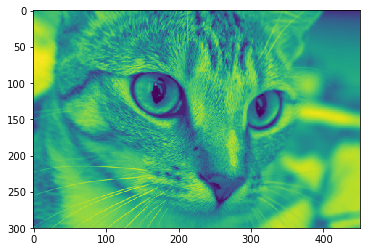
2. Knowing that the image cat is a numpy array with shape 300x451x3, understand the mathematical formula behind the luminance calculation in the code cell below.

weights = np.array([[0.2126], [0.7152], [0.0722] ])
luminance = cat @ weights
plt.imshow(luminance.squeeze())

<matplotlib.image.AxesImage at 0x1a8e45b5cf8>

Takeaways

• Think in shapes; many bugs are shape mismatches.

• Use broadcasting to avoid loops; prefer vectorized operations.

• In linear algebra, @ is matrix product; * is elementwise.

• Prefer solve/lstsq to explicit inverses.

• Transpose/reshape change views of shape; they don’t alter the underlying values.

• Check dimensions early and often; write shapes next to symbols.